The Pivot Table is a tool that Excel uses to create custom reports from your spreadsheet databases. Once you select the portion of your spreadsheet that contains the target data, then define it as a Table and name it, it becomes a Pivot Table, which is subject to all of the Pivot Table tools.
With these tools, you can filter, sort, reorganize, calculate, and summarize one database Table or several Tables. You can extract specific information into a separate, custom report that displays only the relevant information required for your current project.
This article on creating Multi-File Pivot Table Reports is part of a series on Relational Pivot Tables:
- How to create relational tables
- How to create and use filters for date, number, and text fields
- How to create single “flat-file” Pivot Table reports
To make it easier for you to practice the tasks we’re about to describe, we’ve created a downloadable Excel workbook with all the data we use in this article.
The difference between a Single Flat-File Table and Related Multi-File Tables
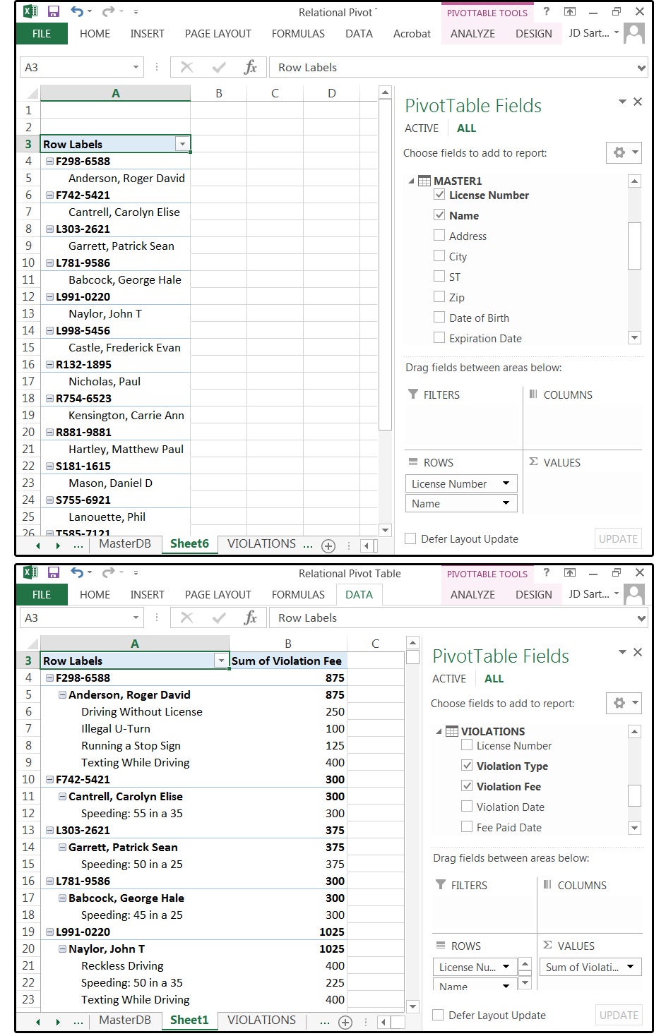
Let's start with a fundamental Pivot Table concept. A single “flat-file” Table is created from a single spreadsheet. Related Multi-File Tables are created from two or more spreadsheets that are connected to one another through a unique key field.
In our sample spreadsheet, the Pivot Table tools allow you to extract the License Numbers and Drivers’ Names from one table (Master1) and the remaining data from another table (Violations). The unique key field, in this case, is License Number, which must exist in all the tables you’re working with for these reports.
As a result, Pivot Tables enable smaller spreadsheets (that is, fewer fields) and eliminate redundant data. Reports are more efficient and easier to compile. For example, in the older versions, you had to enter the client’s name, address, city, state, ZIP code, and phone number in your Client spreadsheet, Product spreadsheet, Sales spreadsheet, Inventory spreadsheet, and more, based on how much data you needed to track that was related to that information. With the Pivot Table tools, you enter data once, then link the tables together through a common, unique field. Excel does the rest.
Related Multi-File Tables: Create relationships
We'll start by showing how you create relationships between multiple spreadsheets for a Pivot Table. Starting in the sample spreadsheet:
 JD Sartain / PC World
Insert / Create PivotTable
1. Access the Violations table.
2. Select Insert > PivotTable.
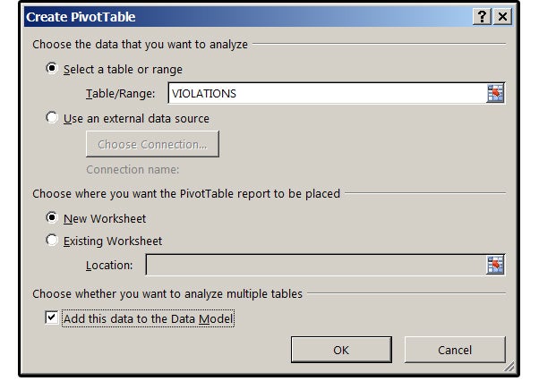
3. In the Create Pivot Table dialog window, ensure that the Table Range says Violations; the location (choose where to place this report) has the New Worksheet circle box checked; and then check the last box: Add this data to the Data Model; and click OK.
Note: The reason we selected the Violations table instead of the Master or Addresses table is because we want to analyze and calculate the data in this table.
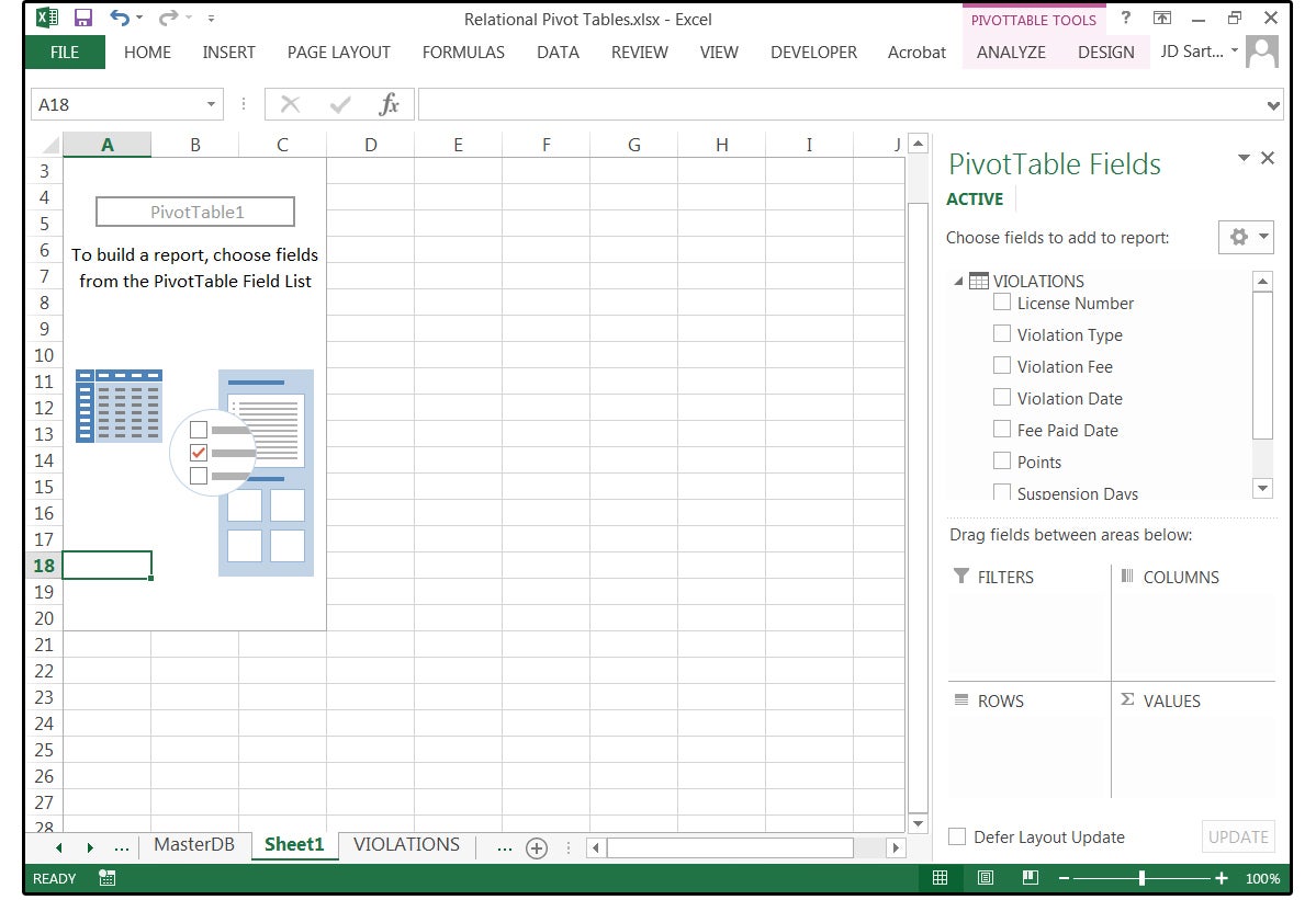
4. The PivotTable Fields panel opens on the right.
 JD Sartain / PC World
The PivotTable Fields panel opens on the right when you're working in this mode.
5. Next, select Data > Relationships, and the Manage Relationships dialog window opens. Click the New button on the right, and the Create Relationship window opens.
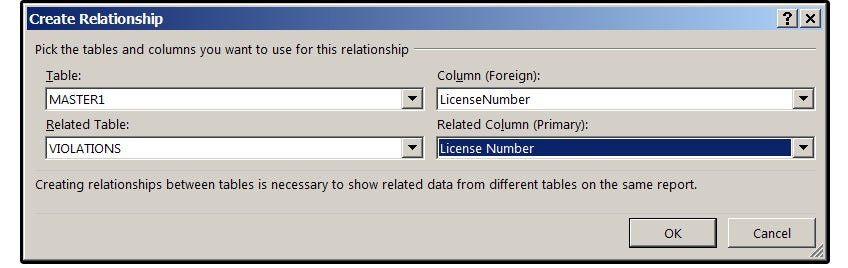
6. Click the down arrow beside the Table field and select Master1 from the list. In the Column (Foreign) Input box, click the arrow and select LicenseNumber from the list.
7. In the Related Table Input box, select the Violations table. Under Related Column (Primary), click the arrow again and select LicenseNumber again from that list.
 JD Sartain / PC World
Create Relationships between the Master1 Table and Violations Table.
8. The Manage Relationships dialog window re-appears. Click the New button on the right and the Create Relationship window opens.
9. Click the down arrow beside the Table field again and select Master1 from the list. In the Column (Foreign) Input box, click the arrow and select LicenseNumber from the list.
 JD Sartain / PC World
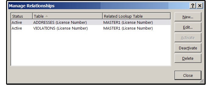
The Manage Relationships window shows two active relationships.
10. In the Related Table Input box, select the Addresses table. Under Related Column (Primary), click the arrow again and select LicenseNumber again
11. The Manage Relationships dialog window re-appears. Notice that you now have two active relationships: Master1 + Violations and Master1 + Addresses. If finished, click OK and then Close.
Create the Pivot Table reports
1. In the PivotTable Fields panel, click the word ALL at the top.
2. Click the Table name arrow to display the fields in each Table. For example, under the Master1 Table, click the LicenseNumber and Name checkboxes.
3. Under Violations Table, click the Violation Type and Violation Fee checkboxes. The PivotTable report appears immediately on the left, growing and expanding as you add more fields.
 JD Sartain / PC World
Select fields from the Master1 Table and fields from the Violations table for this report.
Note: Excel knows which field is the key field, because you defined the relations using the Pivot Table tools in the Create Relationship dialog window. So it’s unnecessary to include the key field (LicenseNumber) in both Tables. If you do, this field will appear twice (in two different areas) in your report. Unless you need it twice in your report, don’t click this field twice. Once in the Master1 table is enough.
Imagine that now your boss wants to see if there is a connection between the violations and the areas (ZIP Codes) where the offending drivers live. You can do this easily.
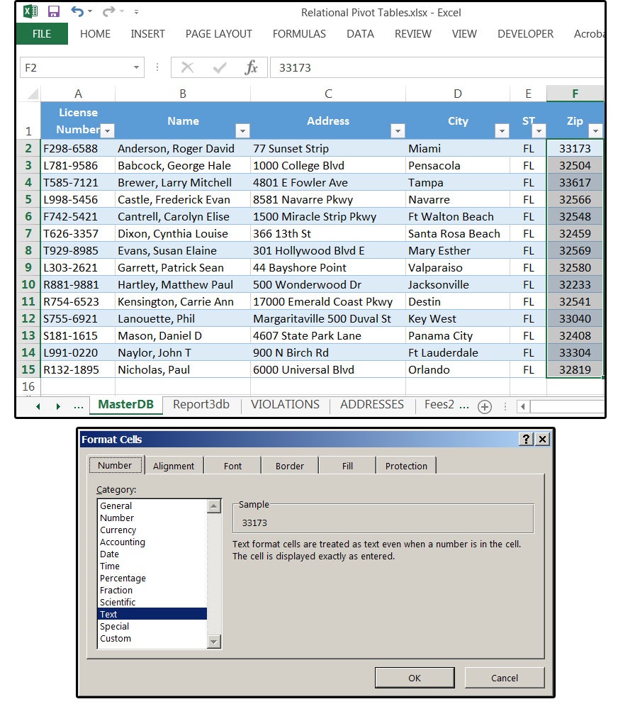
4. First, you must ensure that your ZIP Codes are entered as Text fields. Access the Master1 spreadsheet table and highlight the Zip field.
5. Select Home > Format > Format cells. Under the Number tab, choose Text from the list.
 JD Sartain / PC World
Ensure your ZIP Code field is defined as a Text field.
6. Scroll back to the Master1 Table and click the checkbox beside the field Zip.
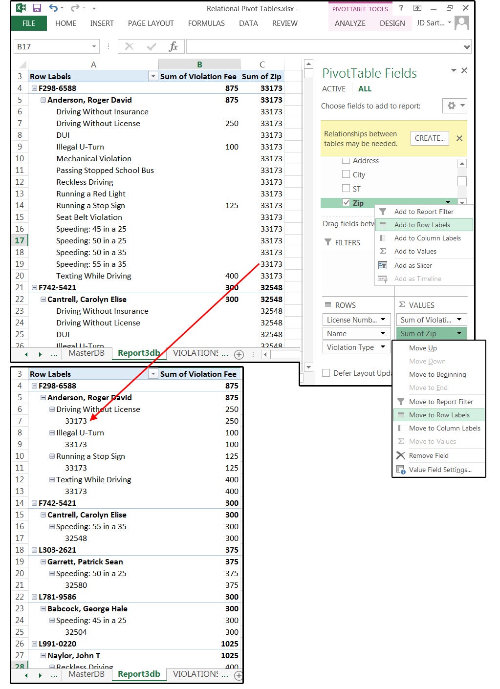
7. A yellow box appears inside your Pivot Table Fields panel that says: Relationships between Tables may be needed, followed by a Create button. If you click this button and re-define the relationships in the Create Relationship dialog window, Excel displays a message that says: A relationship already exists between these two columns. So click Cancel. Save time and just click the 'X' in the upper corner to close the yellow box.
8. If Excel still treats your ZIP Code as a number and places it into a Sum column, right-click the Zip field and choose Move to Row Labels from the drop-down menu list, or go down to the Values box (bottom right of the Pivot Table Fields panel), click the arrow, and choose Move to Row Labels from the popup menu list. And the ZIP Codes move below each violation. Much better.
 JD Sartain / PC World
Close the yellow box, then change ZIP Code to Row Labels.
Next, we’ll add some more fields to enhance our report.
9. Click the Violation Date checkbox under the Violations Table in the Pivot Table Fields panel. Note that Excel adds the dates to columns first, which doesn’t work at all. The data is all over the place and too hard to read.
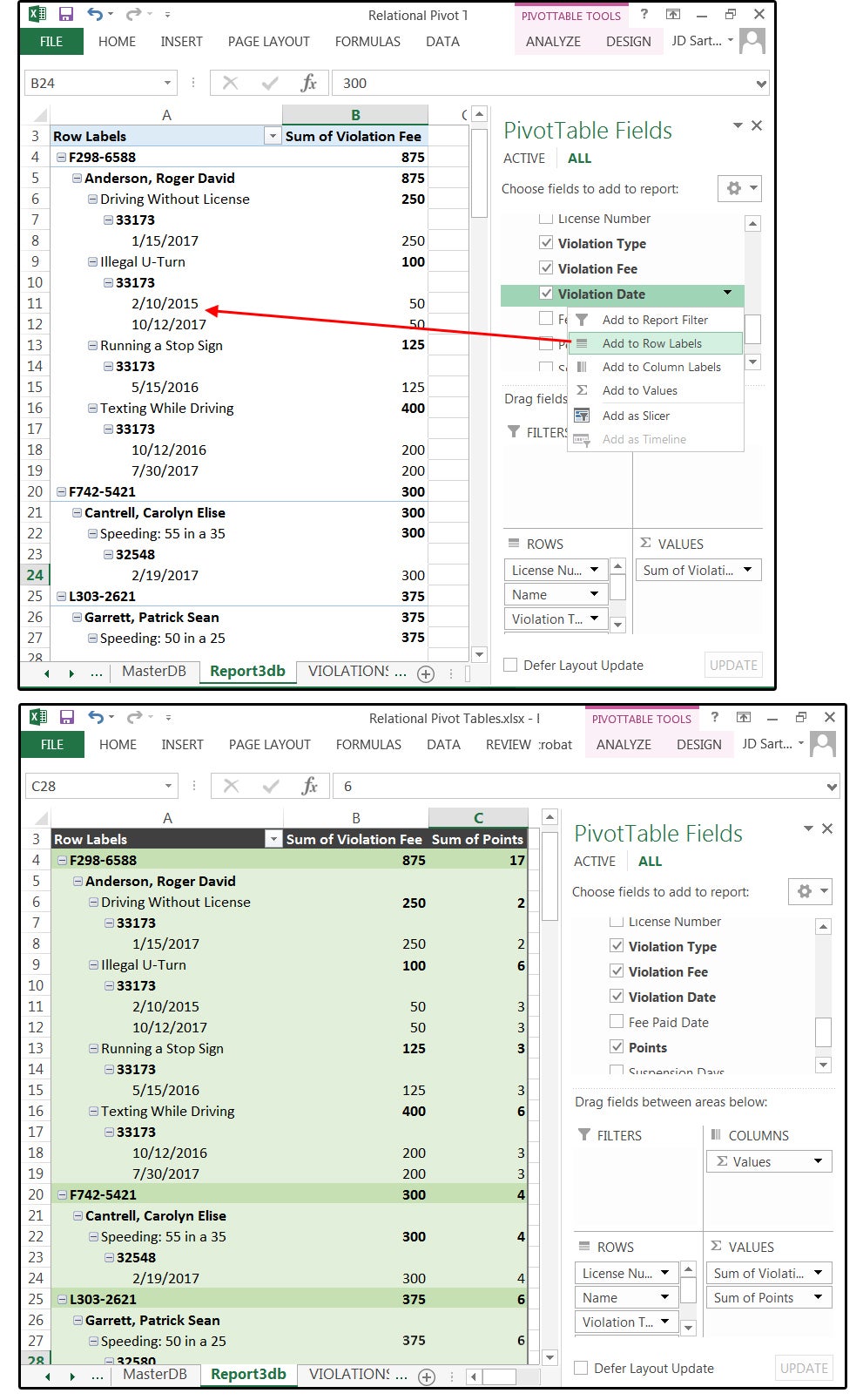
10. Right-click the Violations Date field in the Pivot Table Fields panel (beside the checkbox) and select Move to Row Labels from the drop-down menu list. Notice the date is placed under the ZIP Code and Violation Type. Note that the first driver on the list, Roger David Anderson, has two illegal U-turns, one on Feb 10, 2015, and one on Oct 12, 2017.
11. And last, in the Pivot Table Fields panel, click the Points field under the Violations Table (beside the checkbox).
12. Excel adds the field to your report and sums the points by License Number (by driver) and then also adds a Grand Total for all the Points. Notice how easy it is to add or remove fields to your reports using the Pivot Table tools.
Note: The subtotals and totals are in boldface, and the violations are in regular type. For example, the data on Roger David Anderson’s two illegal U-turns are in regular type, while the U-turns' subtotal of $100 and 6 points is in boldface.
 JD Sartain / PC World
08 Add two more fields to your report: Violation Date and Points
Use the Pivot Table Tools / Design tab (only visible when the report is active) to add color and creative formatting to the Table layout. Tables are easier to read when the rows are alternating colors and the field totals are in bold. Experiment and have fun.
Pivot Table Tips
1. Ensure that you always have more than one spreadsheet in your workbook that’s connected/related to one other spreadsheet through a common, unique field—such as LicenseNumber for our sample.
2. Second, ensure that the Master table has only ONE LicenseNumber per record, which can then connect to several Slave tables that have multiple LicenseNumber records. This is called a one-to-many relationship.
3. Ensure that you have selected and defined all the spreadsheets in your workbook as Tables and given them each unique names.
4. When setting up and defining relationships between tables, the field formats for both of the related tables must be the same. For example, date formats must match—you can't mix '12/25/2018' and 'Dec 25, 2018.'