Microsoft Excel is an incredibly capable and complex spreadsheet program. If you're just getting your feet wet, these tips will help you get started on making a spreadsheet and writing a formula. Once you learn the vocabulary, the rest gets easier.
Open Excel and choose a blank workbook
 JD Sartain / IDG Worldwide
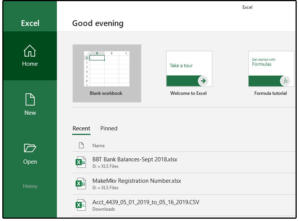
Open a new blank Excel workbook
To get started in Excel, click the Excel icon on your desktop or Start menu. Excel opens with the cursor positioned on the Blank workbook option.
A workbook is the Excel file. All you have to do is click Blank workbook once or press the Enter key, and a blank workbook opens to a blank spreadsheet. You can add spreadsheets to the workbook by clicking the tab with a ‘+’ sign at the bottom of the workbook screen. You can also change the order of spreadsheets in the workbook by sliding their tabs left or right along the tab row. Finally, you can name the tabs as well as name the entire workbook.
Set up an Excel spreadsheet: Columns and fields
The classic spreadsheet format looks just like a bookkeeper’s or accountant’s ledger. Column letters go across the top (these are the fields), and row numbers along the left side (these are records). Think of the traditional calendar format: The days of the week are across the top, and the days of the month that correspond with each day of the week are on the rows beneath the days of the week.
The fields (or columns) are unique data and cannot be repeated—for instance, there cannot be two Thursdays. The records (or rows) are placed beneath the columns. In this example, you could five different days on Thursday in a single month. In a more complicated system, you could have 50 fields with 150 to 5,000 (or more) records in each field.
Excel spreadsheet cells
Every little box in a spreadsheet grid is a cell, which can contain numbers, letters, colors, and formulas. Every field, row, and record resides in its own cell in the Excel spreadsheet.
Each cell is fundamentally defined by its column letter and row number, such as 'Cell A1' for the far upper lefthand corner cell. Check out this earlier story on how to navigate the cells in an Excel spreadsheet.
How Excel Ribbon menus work
The Excel menus (called Ribbon menus) are at the very top of the screen. The tabs across the top are the main menus. Click any of these tabs, and the sub-menus for that tab appear below. The tabs are on a dark-green background, and the selected/active tab turns white.
Now, let’s build a very simple worksheet to show how it’s done.
If you have not moved your cursor since you opened Excel, it currently resides in cell A1. If you have moved it, press the Ctrl+ Home key, which always takes you back to cell A1. Normally, Row 1 is reserved for field/column names. So, type the word Paints in A1, then press the Right arrow and move the cursor to cell B1. Type Colors, press the Right arrow, type # Ordered, press Right arrow, type Cost Each, Right arrow, type Total, then press the Home key.
Notice that in column C, # Ordered is sort of slipping out of cell C1. Let’s fix it.
With your cursor still in the Home position, hold down the Shift key and then press the Right arrow key four times. The Shift key anchors your cursor to the current location; the arrow keys then s-t-r-e-t-c-h out the highlight to the end of the area you want selected.
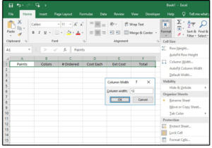
Click the Home tab, then notice that six submenus over is the Cells submenu. Click Format, then choose Column Width from the drop-down list.
In the pop-up box, enter the number 12, then click OK. The columns all widen to accommodate 12 characters.
Adjusting Excel coumn width and row height
The default settings for column width and row height are 8.43 characters wide and 15 high. If you hard-code these settings, you'll have to change them every time you enter a record that exceeds the current column width (or row height).
Instead, use the Autofit settings. Highlight the range, then select Format > Autofit Column Width or Format > Autofit Row Height.
 JD Sartain / IDG Worldwide
Set column width + row height
Cell alignment
While row 1 is still highlighted, click the Home tab again. Notice the stacked lines in the Alignment submenu. The auto-selected option that’s highlighted is Center, Top to Bottom, because the top row is for vertical alignment. The second row is for horizontal alignment. Click the middle set of lines on both top and bottom rows, and the field/column names center horizontally and vertically in each cell.
Save an Excel file
Click the File tab, select Save from the side menu, browse to the location where you want to store this file, name it, then click Save. After the first time you save a file, all you have to do to save it again and again is press the Ctrl+S keyboard shortcut. Check out this past story for more handy Excel keyboard shortcuts.
Enter data in Excel
When entering data in Excel, always enter top to bottom, left to right. Because Excel is, basically, an accountant’s ledger sheet, the bookkeepers always enter numbers top to bottom. When you press the Enter key, the cursor moves down to the next cell, not left or right, because that’s how the old calculators worked.
Enter five paint companies in column A; five colors in column B; five Quantities/# Ordered in column C; and the cost of each paint in column D.
Here's where the fun starts.
Enter formulas in Excel
Excel uses functions, which are predefined formulas, to calculate the numbers on your worksheets. Lucky for all of us, there are over 440, with more being added in every version, not to mention third-party vendors who create Add-In programs with their own unique functions.
Without the functions, Excel would just be a word processor that creates lists. To learn more about Excel functions and formulas, read my past stories, including an Excel formula cheat sheet and a guide to the most popular Excel formulas.
 JD Sartain / IDG Worldwide
A simple basic worksheet
Once you've populated columns A, B, C, and D, position your cursor on cell E2. Type this formula in that cell: =SUM(C2*D2) (the asterisk represents multiplication). Excel calculates the total of the Quantity/# Ordered times the cost of each.
You can also position your cursor on the cell location where you want the answer to appear, then press the + (plus) key (then move your cursor to cell C2), press the asterisk—for multiply—(then move the cursor to cell D2), then press Enter.
Reposition your cursor in cell E2. Press the copy command Ctrl+C (a dashed green line rotates around the selected cell, like an active marquis). Move your cursor down to cell E3. Hold down the Shift key and press the Down arrow key three times, then press Enter.
Excel copies the formula in E2 down to E3 through E6. Move your cursor to cell A2. Press and hold the Shift key, cursor right four times, cursor down four times, then center the text horizontally and vertically from the Alignment submenu under the Home tab.
Select a range of cells in Excel
You can also select a range of cells (the term Excel uses to identify a group of adjacent cells) with your mouse. Place your cursor in cell A2, hold down the left mouse button and drag the highlight to cell E6, then choose your options from the Ribbon.